Figure 4.60. Frequency Domain Tab

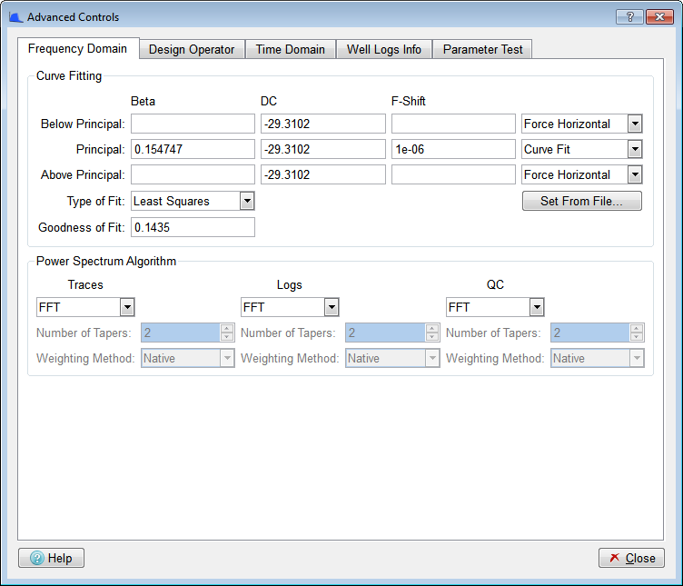
This group is split into the sub-groups "Curve Fitting" and "Power Spectrum Algorithm".

Sub-group: Curve Fitting

This sub-group provides you with control over the curve fitting mechanism. By default, curve fitting is only performed between the "Low Cut" and the "High Cut" frequencies (the primary controls) which are defined in the "Fit Well Log Curves" group on the "Design Controls" dialog. This curve fit is referred to as the "Principle" curve. Below the "Low Cut" and above the "High Cut" we force the curve fit to horizontal, with the value of the "Principle" at the "Low Cut" and "High Cut" points.

Whilst using these advance controls it is advisable to QC the resulting curve fit by always having the spectrum you are trying to fit and the composite curve fit visible on one of the SsbQt Main Window charts (by default the "Global" chart). Immediately you make a change to one or more of the "Frequency Domain" parameters you will see the change on your Main Window chart. Note, it might not be possible to QC against a spectrum if no well data is available. Under such circumstances you would need to supply the curve fit parameters manually or read them from file.

Within the "Curve Fitting" group there is a matrix of "Beta" "DC" and "F-Shift" for "Below principal", "principal" and "Above principal" curves. For each curve there is a combo control to the right which specifies the mode of curve fit. We will now consider each of these three curves and describe their mode of use.

Below principal: The default mode is "Force Horizontal". In this mode, the "Beta", "DC" and "F-Shift" are insensitive and cannot be used. The "DC" value displayed is the value of the "Principal" curve fit at the "Low Cut" point. The "Fit Independently" mode uses the same curve fit algorithm between 0 Hz and "Low Cut" as that used for the "Principal" curve fit. The displayed "Beta", "DC" and "F-Shift" are parameters from the independent fit. This mode frequently gives strange results and its usage is not normally recommended. The "Extrapolate Principall" mode allows the "Principal" curve to be extrapolated, below the "Low Cut", back to 0 Hz. The "Set" mode allows you to manually set the sensitive "Beta", "DC" and "F-Shift" of the "Below principal" curve. However, the "Set" mode is not normally recommended.

Principal: The "Principal" curve is by far the most important curve hence its name. The default mode is "Curve Fit". Curve fitting is performed between the "Low Cut" and the "High Cut" frequencies defined in the "Fit Well Log Curves" group on the "Design Controls" dialog. The "Beta" is the key curve fit parameter and is also displayed on the "Design Controls" dialog. The "Set" mode allows you to manually set the sensitive "Beta", "DC" and "F-Shift" of the "Principal" curve.

Above principal: The default mode is "Force Horizontal". In this mode the "Beta", "DC" and "F-Shift" are insensitive and cannot be used. The "DC" value displayed is the value of the "Principal" curve fit at the "High Cut" point. The "Fit Independently" mode uses the same curve fit algorithm between "High Cut" and nyquist as that used for the "Principal" curve fit. The displayed "Beta", "DC" and "F-Shift" are parameters from the independent fit. This mode frequently gives strange results and its usage is not normally recommended. The "Extrapolate Principal" mode allows the "Principal" curve to be extrapolated beyond the "High Cut" up to nyquist. The "Set" mode allows you to manually set the sensitive "Beta", "DC" and "F-Shift" of the "Above principal" curve. However, the "Set" mode is not normally recommend.

There are two other "Advanced Controls" on the "Frequency Domain" tab "Type of Fit" and "Set From File...". The following described these controls:

Type of Fit: This radio button control allows you to select the type of fit algorithm. Possible values are "Least Squares" or "Robust". By default, the type of fit is "Least Squares".

Set From File...: This push button will pop up a file selector dialog allowing you to read a previously saved session file to load the "Beta", "DC", "F-Shift", curve fit "Low Cut" and curve fit "High Cut". If there is a session file associated with this SsbQt run either via "File->Open..." or "File->Save As..." then that session file will be the default. You can also use this mechanism to load the above parameters from Spectral Blueing V2.3.x saved files. However, it should be noted that it is not possible to load from SsbQt V2.90 session files as these parameters were not saved in that version. This option is useful when no well data is available or you wish to use the same curve fit parameters from a previously saved session.

The field Goodness of Fit displays the correlation coefficient value calculated between the Average Well Logs Spectrum and the Principal Curve Fit between Low and High cuts. Pearson's correlation formula is used to calculate the correlation coefficient.

Sub-group: Power Spectrum Algorithm

This sub-group provides the user control over the power spectrum algorithm. By default, all the spectrum calculations are performed by the FFT (Fast-Fourier Transform) algorithm. The other possible option is the Multitaper algorithm, which was developed by Thomson (1982).

The Multitaper algorithm starts by multiplying the time series data sequence by a set of K orthogonal sequences, also known as tapers, to form a K number of tapered time series, from which are generated K frequency spectrum estimates by using the FFT algorithm, that are finally combined as an estimate of the Power Spectral Density (PSD) function. The orthogonal sequences used to "taper" the time series data sequence are generated by using the Discrete Prolate Spheroidal Wave Functions (DPSWF) algorithm.

There are 2 parameters in this sub-sgroup:

Weighting Method: To estimate the PSD, a set of weights are required and this combo box provides the user the choice of selecting the weighting/combining method. By default, the Native weighting method is used, which averages the spectrum estimates according to their respective eigenvalue, whereas the Adaptive weighting method generates a smooth estimate by reducing the bias from the spectral leakage. The adaptive weighting is an iterative method, which keeps computing the weights until the change in spectrum estimate is less than a pre-defined tolerance.

Number of Tapers: This spinbox allows the user to control the number of tapers when performing the PSD using Multitaper algorithm. By default, the number of tapers allowed is 2 and the maximum number of tapers that can be used to compute the PSD has been set to 50.

Figure 4.61. Design Operator Tab

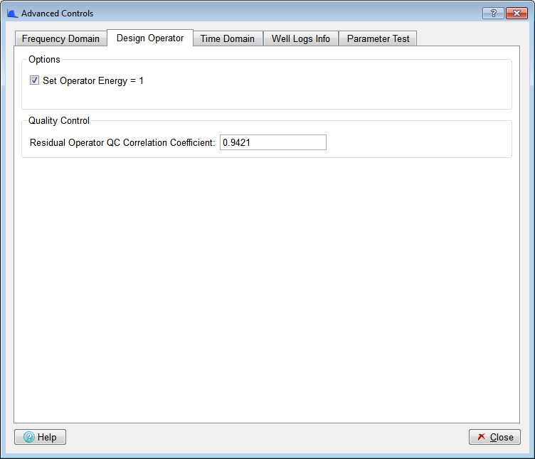
There is currently only one parameter in this group.

The Set Operator Energy = 1 checkbox item is here for backward compatibility with earlier versions of the Spectral Blueing software. This checkbox item allows the time-converted operator to be normalised. With this turned on, the amplitude values are adjusted so that the energy in the time converted operator is set to one.

The field Residual Operator QC Correlation Coefficient displays the correlation coefficient value calculated between the Residual Operator Desired Output and the Convolved Smoothed Average Trace Spectrum. Pearson's correlation formula is used to calculate the correlation coefficient.

Figure 4.62. Time Domain Tab

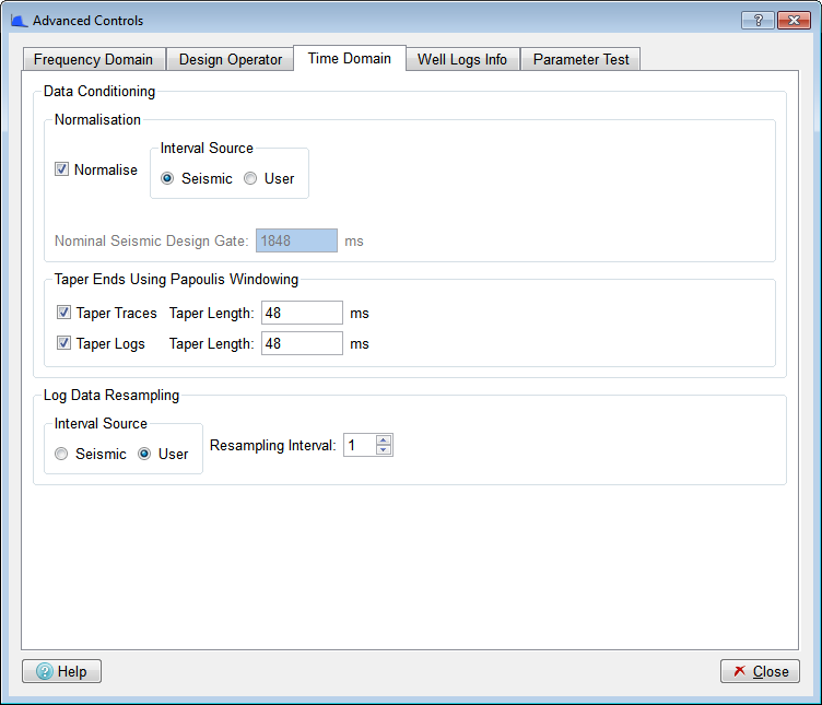
This group is split into the sub-groups "Data Conditioning".

Sub-group: Data Conditioning

For the spectral blueing result to have amplitudes which have physical meaning, then it will be necessary to normalise the Reflectivity log spectral amplitude. This is achieved by compensating for the effects of the relative differences between the seismic and Reflectivity log gate lengths together with the relative differences between the seismic and Reflectivity log sample intervals.

Normalisation

Normalise: This checkbox item allows you to toggle on/off the normalisation facility.

Interval Source: This radio button control allows you to specify whether the Sample Interval or Design Gate is determined from Seismic or User. If the source is Seismic then the normalisation parameters are obtained from the sample interval and gate length of the seismic data. If the source is User then you need to additionally provide the Nominal Seismic Sample Interval (ms) and Nominal Seismic Design Gate (ms) see below.

Nominal Seismic Sample Interval (ms): This spinbox control allows you to specify the nominal seismic sample interval to be used for normalisation purposes. This control is active if User is set for the "Interval Source" radio button above.

Nominal Seismic Design Gate (ms): This line edit field allows you to specify the nominal seismic design gate length to be used for normalisation purposes. This control is active if User is set for the "Interval Source" radio button above.

Taper Ends Using Papoulis Windowing

Taper Traces: This checkbox item turns on the apply taper facility for seismic traces. This allows the ends of the input seismic traces to be tapered.

Taper Length (ms): This input field value allows you to specify the taper length in milliseconds to apply to the input seismic traces

Taper Logs: This checkbox item turns on the apply taper facility for Reflectivity log data. This allows the ends of the input Reflectivity Log data to be tapered (previously referred to as ramped).

Taper Length (ms): This input field value allows you to specify the taper length in milliseconds to apply to the input Reflectivity Log data.

Figure 4.63. Well Logs Info Tab

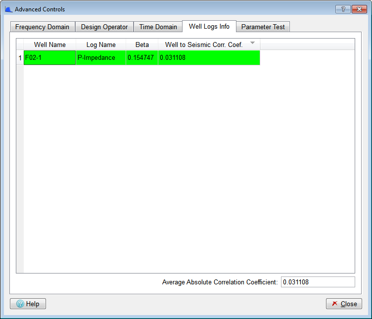
The table on this tab shows, for each of the selected input well logs, the Well to Seismic correlation coefficient value, which is calculated between the filtered well log(the impedance well log convolved with the Band Pass Operator) and the seismic trace nearest the well location. In addition it also displays the Beta (for SCI) or Beta (for SSB) value for each individual well.

The row in light green corresponds to the well log that has highest well to seismic correlation value.

On the bottom right corner you can also see the Average Absolute Correlation Coefficient, which consists of the average of the absolute values of all the correlation values from the table.

Note that if ASCII logs without position information have been used then it is not possible to use these to calculate an Well to Seismic Correlation Coefficient.

Figure 4.64. Parameter Test Tab

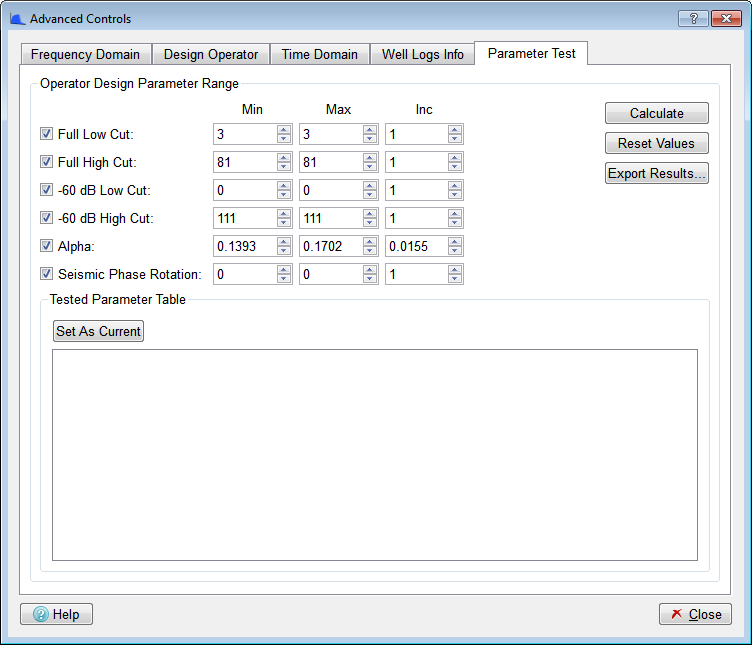
Using this tab it is easy to test how much a change of one or more parameters can affect the calculated operator. A range of candidate values for one or more parameters can be entered, and the effects of these changes can be conveniently viewed.

The parameters that can be adjusted come from the Design Controls Dialog and they consist of:

For each of the parameters mentioned above you can set a minimum, maximum and increment value. You can also include or discard a certain parameter from the test by using the checkbox next to it.

To run the parameter test you must click the Calculate button, and the Residual Operator QC Correlation Coefficient value will be calculated for each combination between different values of all the parameters that are ticked. In the following example Full Low Cut has been requested between the values of 0 and 3 Hz and the Full High Cut between 74 and 85 Hz.

Note that if ASCII logs without position information have been used then it is not possible to use these to calculate an Average Correlation value, so the Correlation column will be filled with zeros.

Figure 4.65. Parameter Test Tab with Full Low Cut range

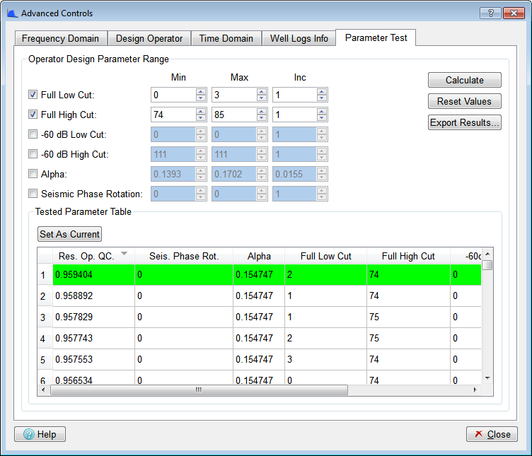
The results for the parameter test are then shown on the table. The row in light green corresponds to the parameters combination that gives the best Residual Operator QC Correlation Coefficient value.

To see the immediate effect of a set of parameters both in the Seismic View, and in the Design Controls panel, click on the row to select it, and then use the Set As Current button (or double-click on the row). The diagram below shows that row 1, with Full Low cut of 2 Hz and Full High Cut of 74 Hz has been selected. The values 2 Hz and 74 Hz can be seen in the Full Low and High Cut fields in the Design Controls panel.

The effect of a row of values can also be seen by double-clicking in that row.

Figure 4.66. Parameter Test Tab used to update Desgin Controls

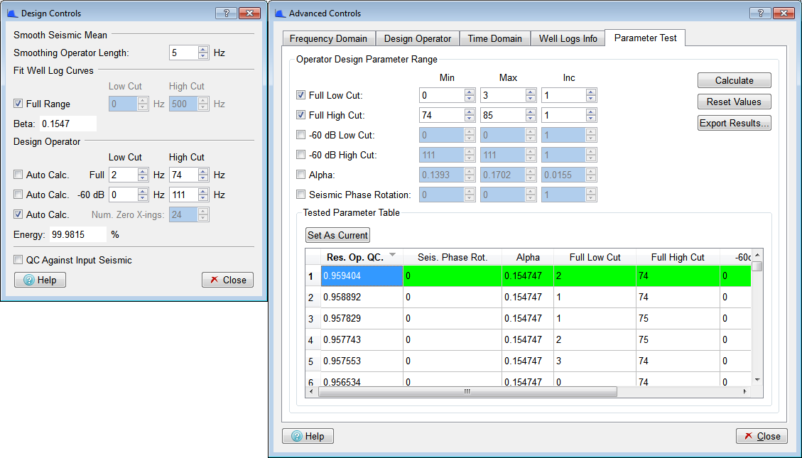
If you want to export the results to a file you can use the Export Results button, which will prompt you for a text file to write them to.

Finally, the button Reset Values can be used to reset each of the parameters to the values present on the Design Controls Dialog.