There is a variety of techniques available to invert seismic data ranging from very simple to complicated. Let's consider two techniques: Parametric Inversion (sparse spike) and Coloured Inversion.
Most inversion algorithms use parametric inversion where the earth is modelled by a series of parameters. Basically parametric inversion works like this:
Start with an initial estimate of all the model parameters.
Define a function that characterises where the current model deviates from a desired model.
Update the model so as to reduce the deviation.
Iterate 2 and 3 until an acceptable error level is reached.
The model parameters are automatically updated to reduce the error term. The error term itself is a weighted sum of a series of different terms. For example:
Seismic misfit term.
Reflection coefficient threshold term.
Deviation from the starting model term.
Trace by trace variation term.
These terms are limited on the expected AI values within specified layers. The model parameterisation together with the constraints and some of the above terms may extend the inversion beyond the bandwidth of the seismic. The most important of the above is the seismic misfit term. In order to generate the seismic misfit term, this form of inversion requires the user to supply an explicit wavelet. This is generally performed prior to performing the inversion itself. The benefit of this is that it forces the user to tie and understand the log seismic fit. However, the downside is the wavelet is affected by calibration errors in the logs. Generation of wavelet is a difficult task and can be error prone.
Coloured Inversion takes a different approach that is more familiar to seismic processing. In simple terms we analyse various seismic and well log spectra to define an operator that shapes the average seismic trace spectra to that of a fitted smooth curve which is representative of the average AI log spectrum. This defines the amplitude spectrum of the required operator. Theory tells us that a 90 degree phase rotation is also required. This is incorporated into the operator. The assumption is that the input seismic data is zero phase. The Coloured Inversion operator is converted to the time domain and simply applied to the seismic volume using a convolution algorithm.
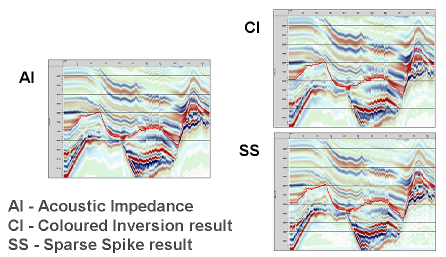
Let us compare a synthetic example. Using model data we can generate synthetic seismogram. In the figure below we see three relative AI displays which are broadly similar. On the left we see the relative AI directly from the input model data. This is the result (i.e. the answer). On the top right is the Coloured Inversion result generated from the synthetic seismogram. On the bottom right is the sparse spike inversion from the same synthetic seismogram.
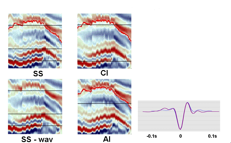
Now if we compare the display above in greater detail we will observe an interesting result. Let's consider the figure below. The top two displays labelled SS (for Sparse Spike) and CI (for Coloured Inversion). On first observation the SS result looks better as it would appear to offer higher resolution. However, if we compare both the SS and CI with the answer AI (bottom right) then it is the CI result which more closely resembles the input model. Why should this be? Tracking down the problem found that the wavelet required by SS was estimated slightly incorrectly (difference between the purple and blue curves in the bottom far right plot.) The original wavelet estimate is deficient at high frequencies, for which the derived AI solution must compensate. When the sparse spike inversion is given the correct wavelet, it gives a similar result to CI. Thus, this example shows how easy it is to get sparse spike inversion wrong even when the answer is known. CI doesn't suffer from this problem as it is not necessary to determine the wavelet.
Below are some real data examples showing the benefits of seismic inversion and, in particular, Coloured Inversion.
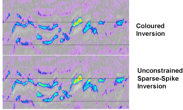
The real data example within the figure shows great similarity between the Coloured Inversion and the unconstrained Sparse Spike result. The advantage of using Coloured Inversion is that the result can be obtained within an hour or two, whereas, Sparse Spike inversion can take several days to perform and uses specialised software that is not available to many interpreters. Furthermore, there is no guarantee that the result will be superior and, as we have shown, if the wavelet is not estimated correctly the result can frequently be worse.
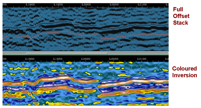
The 3D X-line example in the figure above shows a comparison of Full Offset Stack section (top) and Coloured Inversion section (bottom). It can be seen that interpreting the Coloured Inversion can make it easier to identify events. In particular the fault at L2020 is less likely to have been interpreted using the Full Offset Stack only. In contrast, on the Coloured Inversion section It would be very difficult to miss. This is a good example of how inversion products can help improve interpretation.
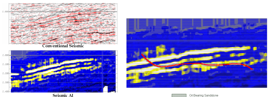
The example in the figure above shows how inversion products using a blue-yellow colour bar can be used in well planning (bottom left). Here the yellow colour indicates pay sands whilst the blue indicates non-pay lithologies. Compare this with the conventional seismic display (top left). The display below shows how a horizontal well can be planned on the basis of seismic inversion. The correspondence between predicted reservoir and actual reservoir is high.